Governments have many goals. To simplify, the two most important kinds of macroeconomic goals can be categorised as external balance and internal balance. Internal balance is the desirable point on the trade-off between output and inflation. To be sure, this trade-off looks different in the long term than in the short term, for well-known reasons. External balance could be defined as a current account at its desirable level.
The Tinbergen (1952) principle remains as valid as ever: to attain N independent goals, a government needs N independent policy instruments. There will always be an important place for models in which N=2, if for no other reason than that we can only draw graphs readily in two-dimensional space. The Meade-Johnson application of the principle (Meade 1951, Johnson 1958) remains useful: to pursue the two goals of internal and external balance, the two most important kinds of instruments are expenditure policies (particularly fiscal and monetary policy) and switching policies (particularly the exchange rate). To be sure, we are less certain as to the effect of a devaluation than we were in the old days of Meade-Mundell-Fleming. This uncertainty is mainly due to some contractionary implications of devaluation,
especially the balance sheet effect of devaluation, which arises if the country has incurred debt denominated in foreign currency. But we can be pretty sure that devaluation raises inflation and thus would have to be offset by spending contraction if the same level of internal balance were to be maintained.
The Meade-Mundell-Fleming framework was based on the assumption that the two most relevant goods are the domestic good, whose price is set in terms of domestic currency, and the foreign good whose price is set in terms of foreign currency. This assumption is the producer currency pricing paradigm (PCP). More recently, the assumption has been challenged by the dominant currency pricing (DCP) paradigm (Gopinath 2015, Gopinath, et al. 2020, Amiti et al. 2022, Itskhoki et al. 2013). The challenge is warranted, in light of the strong empirical evidence that most tradable goods – not just imports but also exports – are invoiced in terms of the dollar or other major foreign currency, and that a devaluation raises the domestic currency price of all these goods, i.e. passthrough is high. The exception is the case of US imports, where passthrough is low. The dollar is, after all, the dominant currency.
This column urges a revival of the Salter-Swan version of the small open economy model (Salter 1959, Swan 1963). Our starting point is a claim that the aforementioned empirical evidence, while consistent with the dominant currency pricing paradigm, is as easily interpreted as consistent with the proposition that the domestic country is a price-taker on world markets for all tradeable goods. This is the case in the long run as well as the short run. That proposition is what it means to be a small open economy (SOE) in trade theory. The country can buy or sell on world markets however much it wants of tradable goods, at the going price.
The small open economy label has been hijacked to characterise other models where the domestic country is small in terms of world financial conditions or global business cycle conditions, but not in global goods markets.
So, I want to be explicit about the price-taker assumption: in the Salter-Swan version of the small open economy model, ‘small and open’ means that the economy is a price-taker on world markets for tradeable goods. The realism of this proposition is not particularly contested in the case of commodities like oil, minerals, or agricultural products. But for many small countries the assumption also applies approximately to some manufactured goods and services, such as apparel, basic consumer electronics, and call centre services.
Simplicity is the aim here. Nevertheless, if all prices of goods and services were exogenous to the small open economy, that would be too simple. To make the model interesting, we want at least two categories of goods and at least one relative price. After having made the price-taker assumption for the tradable goods sector, we have the freedom to focus also on a second sector: non-tradable goods. The tradition of non-traded goods has not died out (e.g. Romei and Fornaro 2022). It is still represented on most graduate reading lists by its application as the Balassa-Samuelson relationship. This relationship is a useful guide to the real exchange rate in long-run equilibrium or across countries. But the Balassa-Samuelson effect – that is, the application of the small open economy assumption to the effect of long-run productivity growth rates on purchasing power parity – has crowded out small open economy models in which one can address spending policy, exchange rate policy, and exogenous terms of trade shocks. Recent textbooks have often left these central macroeconomic issues to the Mundell-Fleming model and its successors.
The Salter-Swan small open economy (SS-SOE) model has other progenitors as well as those two authors. A third Australian, Corden (1960), was among the original SS-SOE wave. Dornbusch (1973, 1974) should also be given credit.
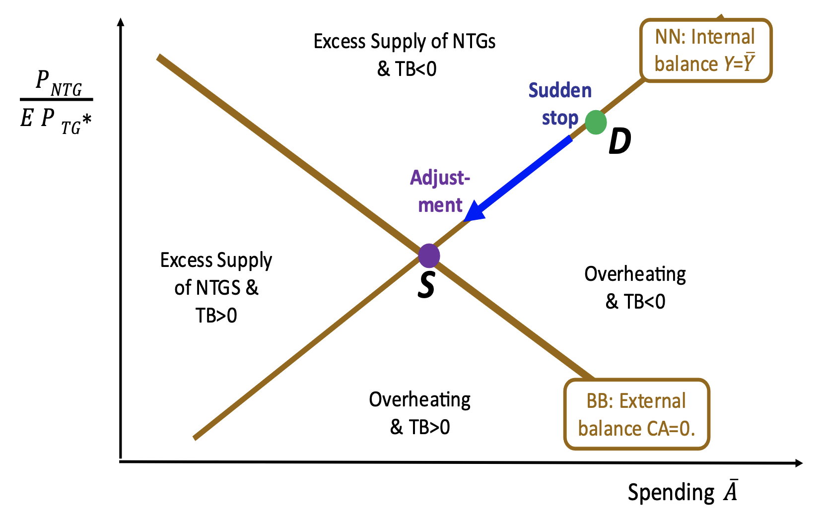
The horizonal axis of the Swan diagram, in Figure 1, represents the level of expenditure. The vertical axis is the relative price of non-traded goods, that is, the ratio of the nominal price of non-traded goods to the exogenous world price of traded goods times the country’s exchange rate.
Or one could define the vertical axis as the reciprocal of that, and call it the real exchange rate. This usage, though not my preference, would define the real exchange rate as the inverse of the relative price of non-traded goods.
Figure 1 The Swan diagram
Note: For example, at D, a CA deficit. A sudden stop of capital inflows calls for adjustment. A combination of devaluation and expenditure reduction returns balance at S.
Four effects
An increase in spending, which is a move to the right in Figure 1, (i) pushes external balance in the direction of current account deficit, and (ii) pushes internal balance in the direction of overheating. A devaluation, a move down in the figure, pushes external balance in the direction of a current account surplus – largely because it incentivises the switching of labour out of the production of non-traded goods and into the production of traded goods, in addition to the usual switching of consumption in the opposite direction. (This will be shown shortly, in the second figure.) And, finally, in the traditional version of the SS-SOE model, devaluation moves internal balance in the overheating direction.
One schedule in the figure, labelled NN, represents combinations of expenditure and the relative price of nontraded goods that are consistent with internal balance. The other schedule, labelled BB, represents combinations that are consistent with external balance. Alternatively, one could map out a complete set of iso-current account lines, to get away from any presumption that the optimal current account is zero.
By way of illustration, Figure 1 shows a country that is running a current account deficit at point D, but now faces a sudden stop of capital inflows. It is forced to adjust. It should undertake a combination of devaluation and expenditure reduction. It can thereby eliminate the deficit at point S, without suffering a recession (excess supply of non-tradable goods) in the process. A recession would be the fate of pure expenditure reduction with no change in relative prices, represented by a move to the left side of the NN schedule.
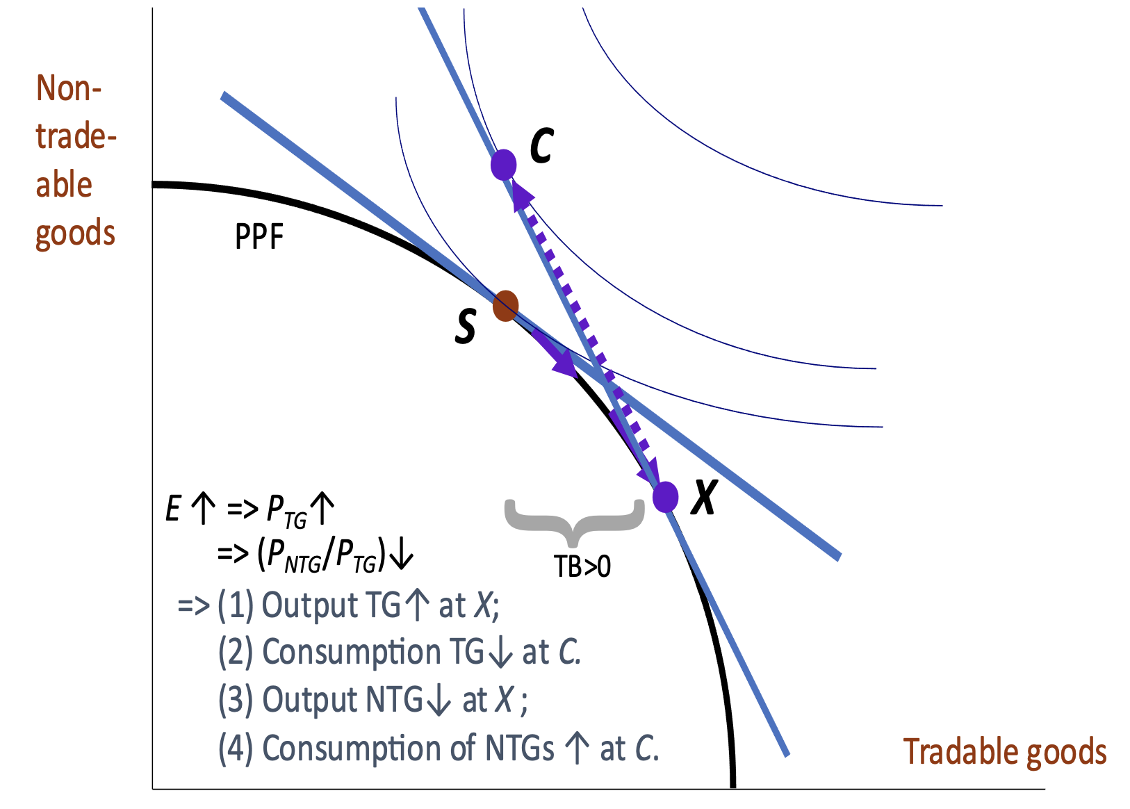
A version of the Swan diagram can be derived in the producer currency pricing framework. But it was originally derived from the model with tradable and non-tradable goods, via the Salter (1959) diagram. Figure 2 shows the elements of the Salter diagram, for the case of a devaluation, starting from full equilibrium at point S: the production possibility frontier between tradables and non-tradables; relative price lines both before the devaluation (the flatter one) and after the devaluation (steepening); production at point S before the devaluation, production at point X after the devaluation, and consumption at point C after. Point C is a point of trade surplus and overheating (inflationary pressure), which in Figure 1 lies in the territory directly below point S.
Figure 2 The Salter diagram
Note: For example, devaluation reduces the relative price of non-tradeable goods (NTGs).
The Salter-Swan small open economy model can be used to think about the effects of standard experiments: a sudden stop, a devaluation, monetary or fiscal expansion, and fixed versus floating exchange rates. Unlike the traditional producer currency pricing model, it can also show the ‘Dutch disease’, which is the effect of a commodity boom for a country that exports oil, minerals, or agricultural products. The commodity boom stretches the production possibility frontier rightward (e.g. Corden and Neary 1982, Sachs 2007).
Commodity exports are very important for most economies in Latin America, Africa, and the Middle East, being the biggest source of shocks. It is in such countries that there is the greatest need for reviving the Salter-Swan small open economy model.
In reality, one could recognise many categories of goods, far more than two, and many relative prices. Six important categories are nontraded goods with sticky prices, nontraded goods with flexible prices, tradable goods in which a given country is a price-taker, tradable goods that are governed by producer currency pricing (PCP), or local currency pricing (LCP), or pricing-to-market (PTM) or dominant currency pricing (DCP). Plus, one needs two tradable goods, if one is to allow for shifts in the terms of trade. When one wants a simplified two-good model, it is a matter of empirical evidence and judgment which two categories of goods are the most useful and what assumption about pricing is the most realistic. Quite likely, different models are useful for different cases, depending on the characteristics of the country in question. I would suggest that for many small countries, especially those where commodities are the most important export, it is possible that the Salter-Swan small open economy model should be the default option.
An influential empirical test of the traded/non-traded goods pricing assumption (versus the producer currency pricing assumption) is Engel (1999). He offered statistical evidence that movements in the real exchange rate are strongly dominated by movements in the relative prices of domestic versus foreign goods, and not by movements in the relative prices of non-traded versus traded goods. One possibility is that the two-good paradigm is a better fit with the US and other major advanced countries, but not for smaller and developing countries (which were not tested in Engel’s paper). Another possible interpretation is that, because prices of imported goods are observed at the retail level, they already include a substantial non-traded domestic component in the form of local transport, marketing and retail (e.g. Burstein et al. 2005), as Engel notes.
Why is the Salter-Swan model disappearing (gradually) from reading lists in graduate economics programmes and (rapidly) from the research frontier?
A major contributing factor is inadequate microeconomic foundations. Figure 2 is pure microeconomics, but has no intertemporal optimisation. Fortunately, Schmitt-Grohé and Uribe (2021) have recently provided a version of Salter-Swan with complete micro-foundations. I hope this enhances the legitimacy of the model.
This leaves us with a lot of scope for empirical testing of the Salter-Swan small open economy model, versus the producer currency pricing and dominant currency pricing alternatives. One place to look is the effect of cross-currency exchange rates. In the dominant currency pricing paradigm, a general appreciation of the dollar against a basket of major currencies should immediately and proportionately raise the price indices of tradable goods that are observed in small countries. If the general appreciation of the dollar has little effect on the price indices of individual countries, their economies may be better described by the SS-SOE model. Another possible place to look is the effect of a devaluation on the quantity of exports versus the output of tradable goods generally.
In any case, the Salter-Swan small open economy model still has a lot of insight to offer.
References
Amiti, M, O Itskhoki and J Konings (2022), “Dominant currencies: How firms choose currency invoicing and why it matters”, The Quarterly Journal of Economics 137(3): 1435-1493.
Burstein, A, M Eichenbaum and S Rebelo (2005), “Large Devaluations and the Real Exchange Rate”, Journal of Political Economy 113(4): 742-784 (also NBER Working Paper 10986).
Chinn, M, X Nong and Y-W Cheudng (2016), “Estimating currency misalignment using the Penn effect: It’s not as simple as it looks”, VoxEU.org, 15 September.
Corden, W M (1960), “The geometric representation of policies to Attain Internal and External balance”, Review of Economic Studies 28(1): 1-22.
Corden, W M and J Peter Neary (1982), “Booming Sector and De-industrialisation in a Small Open Economy”, The Economic Journal 92(368): 825-848.
Dornbusch, R (1973), "Devaluation, Money and Nontraded Goods", The American Economic Review 63(5): 871-880.
Dornbusch, R (1974), “Real and monetary aspects of the effects of exchange rate changes”, in R Z Aliber (ed.), National Monetary Policies and the International Financial System, University of Chicago Press, pp. 64-81.
Dornbusch, R (1976), “Expectations and Exchange Rate Dynamics”, Journal of Political Economy 84(6): 1161-1176.
Engel, C (1999), “Accounting for U.S. Real exchange rate changes”, Journal of Political Economy 107: 507-538.
Frankel, J (2005), "Contractionary Currency Crashes in Developing Countries in Developing Countries", IMF Staff Papers 52(2).
Galí, J and T Monacelli (2005), “Monetary policy and exchange rate volatility in a small open economy”, Review of Economic Studies 72: 707-734.
Gopinath, G (2015), “The international price system”, Jackson Hole conference, Federal Reserve Bank of St. Louis.
Gopinath, G (2017), “Trade: It’s All about the Dollar”, VoxEU.org, 31 May.
Gopinath, G, C Casas, F Diez and P O Gourinchas (2020), “Dominant Currency Paradigm”, American Economic Review 110(3): 677-719.
Itskhoki, O, J Konings and M Amiti (2013), “Why do large movements in exchange rates have small effects on international prices?”, VoxEU.org ,19 February.
Johnson, H (1958), “Toward a General Theory of the Balance of Payments”, Reprinted in R E Caves and H G Johnson (eds.), Readings in International Economics, pp. 374-388, Richard D. Irwin, for the American Economic Association, 1968.
Meade, J (1951), The Theory of International Economic Policy, Volume I: The Balance of Payments, Oxford University Press.
Mundell, R (1963), "Capital Mobility and Stabilization Policy Under Fixed and Flexible Exchange Rates", The Canadian Journal of Economics and Political Science 29(4): 475-485.
Obstfeld, M and K Rogoff (2000), “Perspectives on OECD economic integration: implications for US current account adjustment”, in Global Economic Integration: Opportunities and Challenges, Federal Reserve Bank of Kansas City, pp.169-208.
Romei, F and L Fornaro (2022), “Understanding the global rise in inflation,” VoxEU.org, 27 May.
Sachs, J (2007), “How to Handle the Macroeconomics of Oil Wealth,” in M Humphreys, J D Sachs and J E Stiglitz (eds), Escaping the Resource Curse, Columbia University Press, pp.173-193.
Salter, W E G (1959), “Internal and External Balance – The Role of Price and Expenditure Effects”, Economic Record 35: 226-238.
Schmitt-Grohé, S and M Uribe (2021), “Reviving the Salter-Swan Small Open Economy Model”, Journal of International Economics 130, 103441.
Swan, T (1963), "Longer Run Problems of the Balance of Payments", in H W Arndt and W M Corden (eds.), The Australian Economy, Cheshire, Melbourne.
Tinbergen, J (1952), On the Theory of Economic Policy, North-Holland Publishing Company.


