In June 2022, the 12-month US inflation rate hit a 40-year high at 9%, after averaging 2.2% between 2000 and 2020. At the same time, the US labour market reached exceptionally high levels of tightness (Crump et al. 2022, Michaillat and Saez 2022, Blanchard et al. 2022), providing one explanation for the high reading of inflation. Simultaneously, however, there were spikes in commodity prices and supply chain disruptions, which provide a natural alternative explanation. This has ignited an important debate among economists and policymakers about the relative contribution of supply versus demand in explaining inflation (Di Giovanni 2022a, Shapiro 2022, Ball et al. 2022).
To describe inflation dynamics, macroeconomic models derive a structural relationship between inflation, expectations, supply-side shocks, and demand-side factors, commonly known as the Phillips curve (Phillips 1958). Central banks are typically interested in estimating the effect of demand on inflation, captured by the slope of the Phillips curve.
Estimating the slope of the Phillips curve during and after the pandemic is challenging, as severe demand and supply shocks occurred contemporaneously and within a narrow time frame. Events such as lockdown closures, the Great Resignation, semiconductor shortages, the obstruction of the Panama Canal, oil price shocks, and the endogenous responses of fiscal and monetary policies impacted inflation through multiple channels. Moreover, the period under consideration is short, thus limiting the statistical power of the analysis.
Identifying the slope of the Phillips curve during and after the pandemic
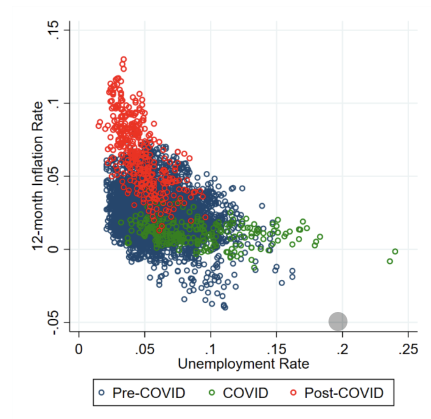
In our paper (Cerrato and Gitti 2022), we estimate the slope of the Phillips curve before, during, and after COVID-19. To do so, we combine the use of panel variation in inflation and unemployment at the US metropolitan area level with an instrumental variable approach. Panel data has the major advantage of increasing sample size for parameter estimation relative to time series analysis based on aggregate data (Mavroeidis et al. 2014). Figure 1 plots the relationship between monthly all-items 12-month inflation and unemployment rates for the 21 MSAs in our sample in the pre-COVID, COVID, and post-COVID periods.
Each data point corresponds to inflation and unemployment rate in a given metropolitan area. A casual look at this figure strongly hints at the flattening of the correlation during the pandemic (shown by green circles) and a steepening thereafter (shown by red circles). Needless to say, while suggestive, the simple correlation shown in Figure 1 could be driven by aggregate and local confounders.
We impose structure on our estimation by proposing a New Keynesian general equilibrium model featuring two regions in a monetary union, along the lines of Beraja et al. (2019) and Hazell et al. (2022). Unlike those papers, we account for the supply-side drivers of COVID and post-COVID inflation dynamics. To do so, we allow for shifts in labour supply preferences and outline a vertically linked production structure consisting of an international commodity market, a national perfectly competitive intermediate-input market, and local monopolistically competitive final-goods markets. Within this setting, we derive regional Phillips curves and relate them to their aggregate counterpart. A key conclusion is that, under reasonable assumptions, the two slopes coincide.
Figure 1 The Phillips correlation across US cities
Notes: The scatter plot shows the relationship between the monthly 12-month all-items inflation rate and the unemployment rate for the 21 US metropolitan areas included in our sample. The blue dots denote observations belonging to the pre-COVID period (i.e., January 1990-February 2020), the green dots denote observations belonging to the COVID period (i.e., March 2020-February 2021), and the red dots denote observations belonging to the post-COVID period (i.e., March 2021-September 2022).
Combining panel data with an instrumental variable approach is essential to identify the slope of the regional Phillips curve. Time fixed effects absorb aggregate shocks (changes in long-run inflation expectations, endogenous policy responses, etc.), and MSA fixed effects control for local structural characteristics, allowed to shift across the three periods (e.g. changes in MSA-level natural unemployment rate). To isolate demand-driven fluctuations in local unemployment rates from local labour supply shocks, we construct a shift-share instrument that captures labour demand shocks in the intermediate input sectors.
The Phillips curve before, during, and after COVID
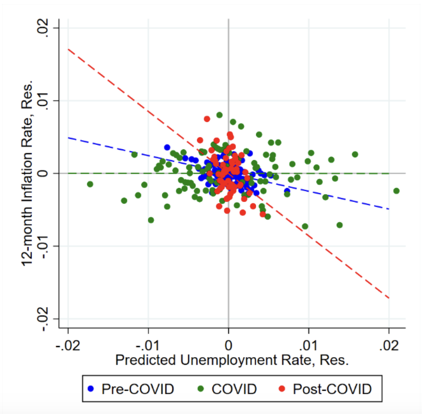
Our benchmark estimates imply a notable flattening of the Phillips curve during COVID and a more than threefold steepening relative to pre-COVID in the aftermath of the pandemic (Figure 2). Considering the estimates provided by the literature for periods prior to 1990 (e.g. Hazell et al. 2022), we conclude that the US Phillips curve has recently been steeper than at any time since the late 1970s. We find that the slope of the Phillips curve increased more distinctively in the early post-COVID phase (i.e. March 2021 to March 2022) and has recently experienced a reversion toward pre-pandemic levels.
The flattening of the Phillips curve during COVID is driven mainly by services, while the subsequent steepening is driven mainly by goods. Moreover, the slope of the Phillips curve exhibits the same dynamic documented in Figure 2 when we exclude the food, energy, and shelter components of the CPI from our inflation measure.
Figure 2 Benchmark estimates of the slope of the Phillips curve
Notes. This figure provides a graphical representation of our benchmark estimates of the slope of the Phillips curve before, during, and after COVID. The figure plots binned residuals from a regression of the 12-month inflation rate on MSA fixed effects, year-quarter fixed effects, the relative intermediate input price, and the final good shift-share control variable against binned residuals of the same specification with predicted unemployment rate as dependent variable. Blue, green, and red dots denote observations belonging to the pre-COVID, COVID, and post-COVID samples, respectively. The dashed lines represent the best linear fits in the three periods, showing the flattening of the Phillips curve during COVID and its steepening after COVID, relative to before COVID.
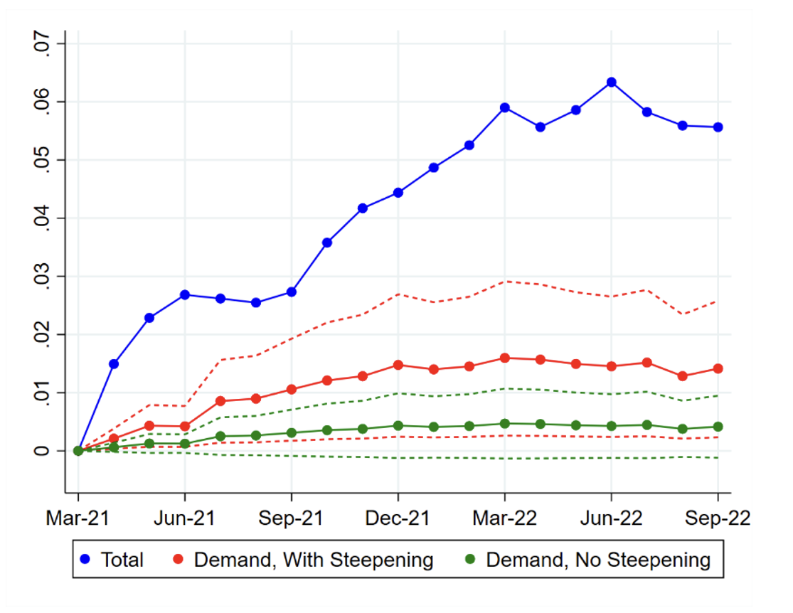
According to our estimates, demand factors explain about one-fourth of the post-COVID increase in CPI inflation. Between March 2021 and September 2022, inflation increased by 5.6 percentage points (Figure 3, blue line), while the unemployment gap
decreased by 1.7 percentage points. Multiplying the change in the unemployment gap (i.e. 1.7%) by our benchmark estimate of the slope of the Phillips curve (i.e. 0.85), we obtain an estimate of the change in inflation imputable to demand factors (i.e. 1.7% x 0.82 = 1.4%, Figure 3, red line). The remaining variation is attributable to shifts in long-run inflation expectations and supply-side shocks.
Had the slope of the Phillips curve not steepened after COVID, the demand contribution to the rise in inflation would have been small and statistically insignificant. Indeed, the same decrease in the unemployment gap would have explained only about 0.4 (= 1.7% x 0.25) of the 5.6 percentage-point increase in inflation, had the slope of the Phillips curve remained unchanged (Figure 3, green line).
Figure 3 Demand contribution to the change in inflation, relative to March 2021
Notes. The figure shows the evolution of the 12-month all-items inflation rate (i.e., blue line) between March 2021 and August 2022, the demand-driven component of this increase with no steepening (i.e., green line) and with steepening (i.e., red line) of the post-COVID Phillips curve, as reported by our benchmark estimates.
References
Ball, L, D Leigh and P Mishra (2022), “Understanding US Inflation during the COVID Era”, NBER Working Paper 30613.
Blanchard, O J, A Domash and L H Summers (2022), “Bad News for the Fed from the Beveridge Space”, Peterson Institute for International Economics.
Crump, R, S Eusepi, M Giannoni and A Şahin (2022), “The Unemployment-Inflation Trade-off Revisited: The Phillips Curve in COVID Times”, NBER Working Paper 29785.
Di Giovanni, J (2022), “How Much Did Supply Constraints Boost US Inflation?”, Liberty Street Economics, Federal Reserve Bank of New York.
Hazell, J, J Herreno, E Nakamura and J Steinsson (2022), “The Slope of the Phillips Curve: Evidence from US States”, The Quarterly Journal of Economics 137(3).
Mavroeidis, S, M Plagborg-Møller and J H Stock (2014), “Empirical Evidence on Inflation Expectations in the New Keynesian Phillips Curve”, Journal of Economic Literature 52(1).
Michaillat, P and E Saez (2022), “u* = √uv”, NBER Working Paper 30211.
Phillips, A W (1958), “The Relation Between Unemployment and the Rate of Change of Money Wage Rates in the United Kingdom, 1861-1957”, Economica 25(100).
Shapiro, A H (2022), “How Much do Supply and Demand Drive Inflation?”, FRBSF Economic Letters, Federal Reserve Bank of San Francisco.
